---
title: "Model Pengukuran (CFA)"
---
```{r}
#| label: setup
#| echo: false
source("_common.R")
```
Bagian ini menyajikan model pengukuran final (CFA) untuk ketiga konstruk: **PEB** (Bifaktor), **OL** (Second-Order), dan **CCS** (Bifaktor).
## CFA PEB — Model Bifaktor {#sec-cfa-peb}
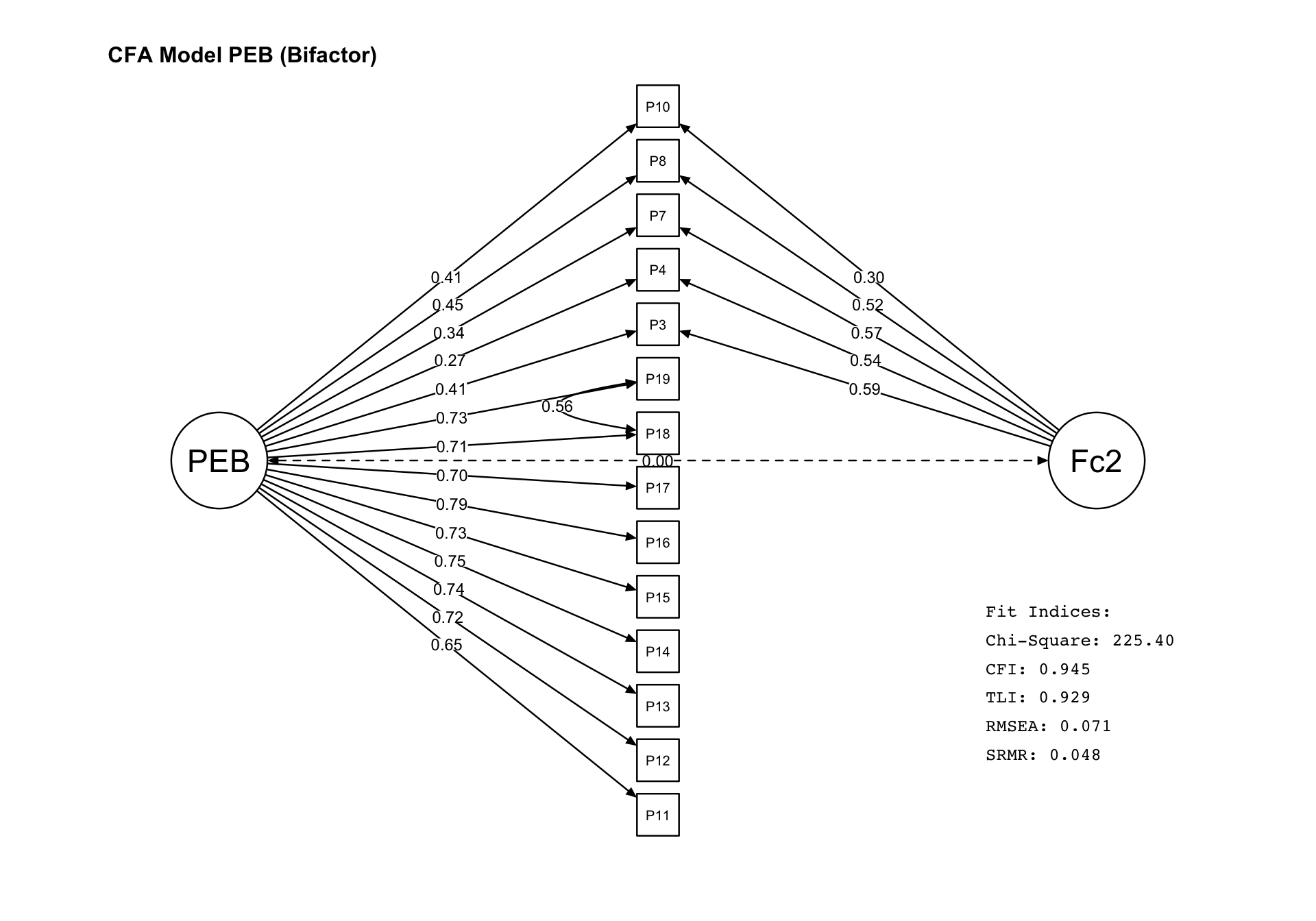
Model bifaktor: satu faktor **umum** (PEB) menjelaskan semua item, ditambah satu faktor **spesifik** (Factor2) untuk item PEB Privat. Faktor umum dan spesifik bersifat **ortogonal**.
> **Referensi**: Brown, T. A. (2015). *Confirmatory Factor Analysis for Applied Research* (2nd ed.).
### Spesifikasi & Estimasi
```{r}
#| label: peb-model
model_peb <- "
PEB     =~ P3 + P4 + P7 + P8 + P10 + P11 + P12 + P13 + P14 + P15 + P16 + P17 + P18 + P19
Factor2 =~ P3 + P4 + P7 + P8 + P10
P18 ~~ P19
"
fit_peb <- cfa(model_peb, data = data, estimator = "mlr",
               orthogonal = TRUE, std.lv = TRUE)
summary(fit_peb, fit.measures = TRUE, standardized = TRUE)
```
### Path Diagram PEB
```{r}
#| label: cfa-peb-plot
#| fig-width: 10
#| fig-height: 7
semPaths(fit_peb, title = FALSE, whatLabels = "std.all", edge.label.cex = 0.6,
         color = "white", edge.color = "black", sizeMan = 3.5, sizeLat = 8,
         layout = "tree2", rotation = 2, bifactor = "PEB",
         style = "lisrel", curve = 2.5, asize = 2, residuals = FALSE, mar = c(3,5,3,5))
title("CFA Model PEB (Bifactor)", cex.main = 1.0, font.main = 2, adj = 0)
fit_idx <- fitMeasures(fit_peb, c("chisq.scaled","cfi.robust","tli.robust","rmsea.robust","srmr"))
op <- par(family = "mono")
legend("bottomright", inset = c(0.1, 0.15), legend = c(
    "Fit Indices:", sprintf("Chi-Square: %.2f", fit_idx["chisq.scaled"]),
    sprintf("CFI: %.3f", fit_idx["cfi.robust"]), sprintf("TLI: %.3f", fit_idx["tli.robust"]),
    sprintf("RMSEA: %.3f", fit_idx["rmsea.robust"]), sprintf("SRMR: %.3f", fit_idx["srmr"])
), bty = "n", cex = 0.8); par(op)
```
### Reliabilitas PEB
```{r}
cat("Cronbach's Alpha:\n"); compRelSEM(fit_peb, return.total = TRUE, tau.eq = TRUE)
cat("\nMcDonald's Omega:\n"); compRelSEM(fit_peb, return.total = TRUE, tau.eq = FALSE)
cat("\nAVE:\n"); AVE(fit_peb)
```
---
## CFA OL — Model Second-Order {#sec-cfa-ol}
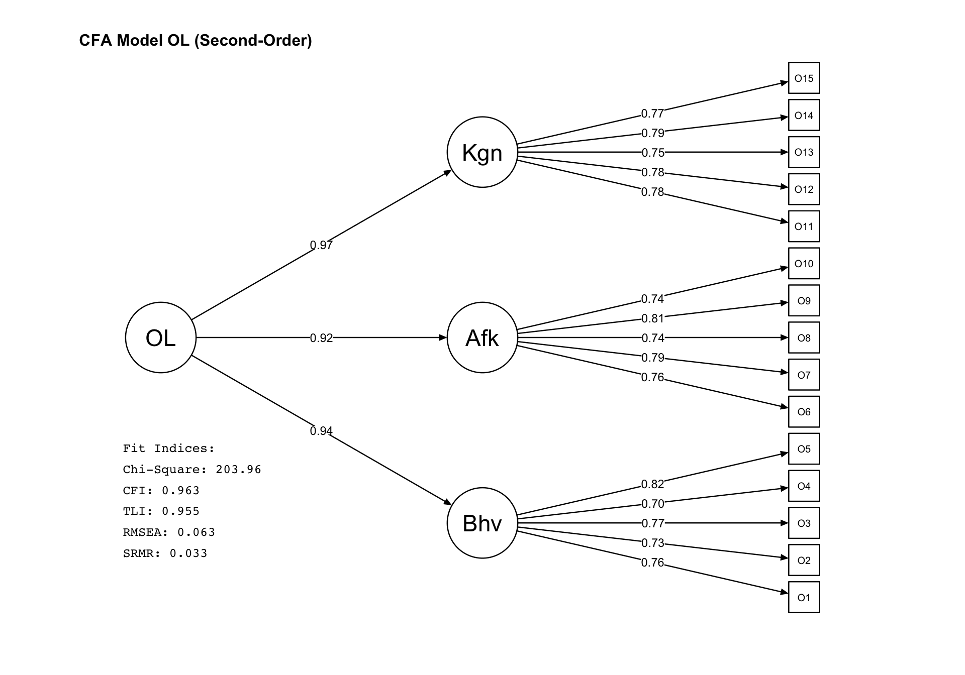
Model second-order: faktor orde pertama (Behavior, Afektif, Kognitif) dan faktor orde kedua (OL) menjelaskan korelasi di antara ketiganya.
### Spesifikasi & Estimasi
```{r}
model_ol <- "
Behavior =~ O1 + O2 + O3 + O4 + O5
Afektif  =~ O6 + O7 + O8 + O9 + O10
Kognitif =~ O11 + O12 + O13 + O14 + O15
OL       =~ Behavior + Afektif + Kognitif
"
fit_ol <- cfa(model_ol, data = data, estimator = "mlr", orthogonal = FALSE, std.lv = TRUE)
summary(fit_ol, fit.measures = TRUE, standardized = TRUE)
```
### Path Diagram OL
```{r}
#| label: cfa-ol-plot
#| fig-width: 10
#| fig-height: 7
semPaths(fit_ol, title = FALSE, whatLabels = "std.all", edge.label.cex = 0.6,
         color = "white", edge.color = "black", sizeMan = 3.5, sizeLat = 8,
         layout = "tree2", rotation = 2, style = "lisrel",
         curve = 2.5, asize = 2, residuals = FALSE, mar = c(3,5,3,5))
title("CFA Model OL (Second-Order)", cex.main = 1.0, font.main = 2, adj = 0)
fit_idx <- fitMeasures(fit_ol, c("chisq.scaled","cfi.robust","tli.robust","rmsea.robust","srmr"))
op <- par(family = "mono")
legend("bottomleft", inset = c(0.1, 0.15), legend = c(
    "Fit Indices:", sprintf("Chi-Square: %.2f", fit_idx["chisq.scaled"]),
    sprintf("CFI: %.3f", fit_idx["cfi.robust"]), sprintf("TLI: %.3f", fit_idx["tli.robust"]),
    sprintf("RMSEA: %.3f", fit_idx["rmsea.robust"]), sprintf("SRMR: %.3f", fit_idx["srmr"])
), bty = "n", cex = 0.8); par(op)
```
### Reliabilitas OL
```{r}
cat("Cronbach's Alpha:\n"); compRelSEM(fit_ol, return.total = TRUE, tau.eq = TRUE)
cat("\nMcDonald's Omega:\n"); compRelSEM(fit_ol, return.total = TRUE, tau.eq = FALSE)
cat("\nAVE:\n"); AVE(fit_ol)
```
---
## CFA CCS — Model Bifaktor {#sec-cfa-ccs}
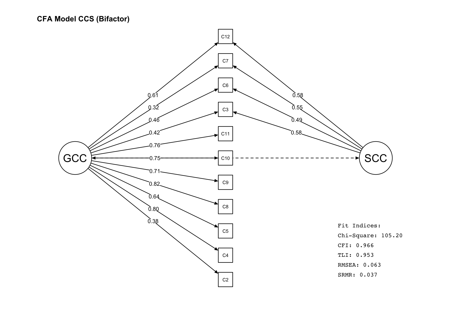
Model bifaktor CCS: *general factor* (GCCS) + *specific factor* (SCCS).
### Spesifikasi & Estimasi
```{r}
model_ccs <- "
GCCS =~ C2 + C3 + C4 + C5 + C6 + C7 + C8 + C9 + C10 + C11 + C12
SCCS =~ C3 + C7 + C6 + C12
"
fit_ccs <- cfa(model_ccs, data = data, estimator = "mlr", orthogonal = TRUE, std.lv = TRUE)
summary(fit_ccs, fit.measures = TRUE, standardized = TRUE)
```
### Path Diagram CCS
```{r}
#| label: cfa-ccs-plot
#| fig-width: 10
#| fig-height: 7
semPaths(fit_ccs, title = FALSE, whatLabels = "std.all", edge.label.cex = 0.6,
         color = "white", edge.color = "black", sizeMan = 3.5, sizeLat = 8,
         layout = "tree2", rotation = 2, bifactor = "GCCS",
         style = "lisrel", curve = 2.5, asize = 2, residuals = FALSE, mar = c(3,5,3,5))
title("CFA Model CCS (Bifactor)", cex.main = 1.0, font.main = 2, adj = 0)
fit_idx <- fitMeasures(fit_ccs, c("chisq.scaled","cfi.robust","tli.robust","rmsea.robust","srmr"))
op <- par(family = "mono", xpd = NA)
legend("bottomright", inset = c(0.1, 0.1), legend = c(
    "Fit Indices:", sprintf("Chi-Square: %.2f", fit_idx["chisq.scaled"]),
    sprintf("CFI: %.3f", fit_idx["cfi.robust"]), sprintf("TLI: %.3f", fit_idx["tli.robust"]),
    sprintf("RMSEA: %.3f", fit_idx["rmsea.robust"]), sprintf("SRMR: %.3f", fit_idx["srmr"])
), bty = "n", cex = 0.8); par(op)
```
### Reliabilitas CCS
```{r}
cat("Cronbach's Alpha:\n"); compRelSEM(fit_ccs, return.total = TRUE, tau.eq = TRUE)
cat("\nMcDonald's Omega:\n"); compRelSEM(fit_ccs, return.total = TRUE, tau.eq = FALSE)
cat("\nAVE:\n"); AVE(fit_ccs)
```