Call:
lm(formula = PEB ~ CCS * OL, data = data_Fscores)

Residuals:
     Min       1Q   Median       3Q      Max
-2.41712 -0.54533 -0.08095  0.52346  2.64555

Coefficients:
            Estimate Std. Error t value Pr(>|t|)
(Intercept) 0.007934   0.037697   0.210    0.833
CCS         0.222501   0.040337   5.516 5.41e-08 ***
OL          0.439350   0.039405  11.150  < 2e-16 ***
CCS:OL      0.038685   0.040248   0.961    0.337
---
Signif. codes:  0 '***' 0.001 '**' 0.01 '*' 0.05 '.' 0.1 ' ' 1

Residual standard error: 0.8532 on 534 degrees of freedom
Multiple R-squared:  0.2038,    Adjusted R-squared:  0.1993
F-statistic: 45.55 on 3 and 534 DF, p-value: < 2.2e-166 Uji Hipotesis Utama
Bagian ini menyajikan uji hipotesis utama (regresi moderasi + HC3) beserta uji asumsi dan plot diagnostik.
- H1: CCS berpengaruh terhadap PEB (efek utama)
- H2: OL memoderasi hubungan CCS terhadap PEB (efek interaksi)
Model: PEB = b₀ + b₁·CCS + b₂·OL + b₃·(CCS × OL) + ε
6.1 Model Regresi OLS
6.2 Hasil Regresi dengan Koreksi HC3
PentingHasil Utama yang Dilaporkan
HC3 (Hayes & Cai, 2007): koreksi standard error yang robust terhadap heteroskedastisitas.
t test of coefficients:

             Estimate Std. Error t value  Pr(>|t|)
(Intercept) 0.0079345  0.0384514  0.2064    0.8366
CCS         0.2225008  0.0418690  5.3142 1.576e-07 ***
OL          0.4393499  0.0440298  9.9785 < 2.2e-16 ***
CCS:OL      0.0386847  0.0504116  0.7674    0.4432
---
Signif. codes:  0 '***' 0.001 '**' 0.01 '*' 0.05 '.' 0.1 ' ' 1
6.3 Uji Asumsi Klasik
6.3.1 Normalitas Residual
Shapiro-Wilk:
    Shapiro-Wilk normality test

data:  residuals(model_reg_peb)
W = 0.99181, p-value = 0.0046
Anderson-Darling:
    Anderson-Darling normality test

data:  residuals(model_reg_peb)
A = 1.5146, p-value = 0.0006607
6.3.2 Homoskedastisitas — Breusch-Pagan
6.4 Plot Diagnostik Regresi
Kode plot diagnostik
diag_df <- data.frame(
    obs = seq_len(nobs(model_reg_peb)), fitted = fitted(model_reg_peb),
    residuals = residuals(model_reg_peb), stdres = rstandard(model_reg_peb),
    leverage = hatvalues(model_reg_peb), cooksd = cooks.distance(model_reg_peb),
    sqrt_abs_stdres = sqrt(abs(rstandard(model_reg_peb)))
)
n_label <- 3; cook_thresh <- 4 / nrow(diag_df)
flag_ids <- unique(c(order(diag_df$cooksd, decreasing=TRUE)[1:n_label],
                      order(diag_df$leverage, decreasing=TRUE)[1:n_label],
                      order(abs(diag_df$stdres), decreasing=TRUE)[1:n_label]))
diag_df$pt_label <- ifelse(diag_df$obs %in% flag_ids, as.character(diag_df$obs), "")
diag_df$influential <- diag_df$cooksd > cook_thresh

qq_df <- diag_df[order(diag_df$stdres), ]
qq_df$theoretical <- qnorm(ppoints(nrow(qq_df)))
qq_extreme <- c(1:n_label, (nrow(qq_df)-n_label+1):nrow(qq_df))
qq_df$qq_label <- ifelse(seq_len(nrow(qq_df)) %in% qq_extreme, as.character(qq_df$obs), "")

sci_theme <- theme_bw(base_size = 11) +
    theme(plot.title = element_text(face = "bold", size = 11, hjust = 0.5),
          plot.subtitle = element_text(size = 9, hjust = 0.5, color = "grey40"),
          axis.title = element_text(face = "bold"), panel.grid.minor = element_blank(),
          legend.position = "none")
col_pt <- "#3A7EBA"; col_ref <- "#C0392B"; col_hi <- "#E67E22"

p1 <- ggplot(diag_df, aes(fitted, residuals)) +
    geom_hline(yintercept=0, linetype="dashed", color="grey40") +
    geom_point(aes(color=influential), alpha=0.65, size=1.8) +
    geom_smooth(method="loess", formula=y~x, se=TRUE, color=col_ref, fill=col_ref, alpha=0.12) +
    scale_color_manual(values=c("FALSE"=col_pt,"TRUE"=col_hi)) +
    labs(title="Residuals vs. Fitted", subtitle="Linearity & Homoscedasticity",
         x="Fitted Values", y="Residuals") + sci_theme

p2 <- ggplot(qq_df, aes(theoretical, stdres)) +
    geom_abline(intercept=0, slope=1, linetype="dashed", color=col_ref) +
    geom_point(color=col_pt, alpha=0.65, size=1.8) +
    labs(title="Normal Q-Q Plot", subtitle="Normality of Residuals",
         x="Theoretical Quantiles", y="Standardized Residuals") + sci_theme

p3 <- ggplot(diag_df, aes(fitted, sqrt_abs_stdres)) +
    geom_point(aes(color=influential), alpha=0.65, size=1.8) +
    geom_smooth(method="loess", formula=y~x, se=TRUE, color=col_ref, fill=col_ref, alpha=0.12) +
    scale_color_manual(values=c("FALSE"=col_pt,"TRUE"=col_hi)) +
    labs(title="Scale-Location", subtitle="Homoscedasticity",
         x="Fitted Values", y=expression(sqrt("|Std. Residuals|"))) + sci_theme

p4 <- ggplot(diag_df, aes(leverage, stdres)) +
    geom_hline(yintercept=c(-2,0,2), linetype=c("dashed","solid","dashed"),
               color=c("grey55",col_ref,"grey55")) +
    geom_point(aes(size=cooksd, color=influential), alpha=0.70) +
    scale_color_manual(values=c("FALSE"=col_pt,"TRUE"=col_hi)) +
    scale_size_continuous(range=c(1,5.5)) +
    labs(title="Residuals vs. Leverage", subtitle="Influential Observations",
         x="Leverage", y="Standardized Residuals") + sci_theme

ggpubr::ggarrange(p1, p2, p3, p4, ncol=2, nrow=2) |>
    ggpubr::annotate_figure(top = ggpubr::text_grob(
        "Regression Diagnostic Plots \u2014 Model PEB", face="bold", size=13))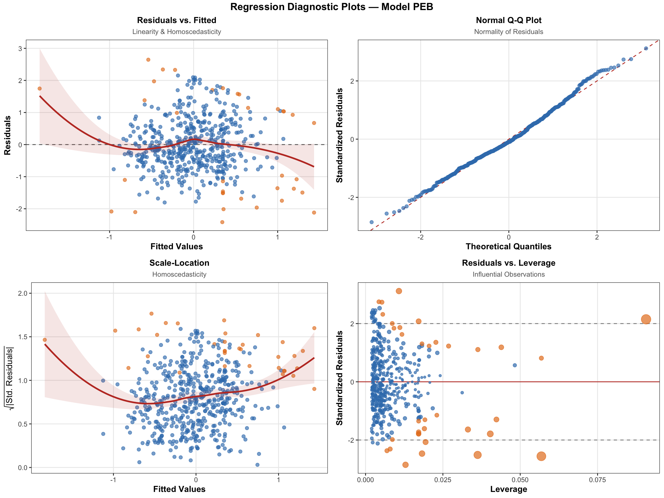
6.4.1 Ringkasan Diagnostik
Max Cook's D: 0.114898 (threshold 4/n = 0.007435)Kode
Obs > threshold: 35 dari 538 (6.5%)
TipInterpretasi
- Residuals vs Fitted: garis horizontal = linieritas terpenuhi
- Q-Q Plot: titik di diagonal = normalitas terpenuhi
- Scale-Location: horizontal = homoskedastisitas terpenuhi
- Residuals vs Leverage: dalam batas Cook’s D = tidak ada outlier berpengaruh